Chapter 3 Materials and methods

3.1 Dataset

The 283 throat swab samples of patients with respiratory symptoms were collected and sequenced between Oct 2019 and Dec 2020. All samples were prepared and sequenced according to the same protocol (github.com/medvir/virome-protocols v2.2.1).

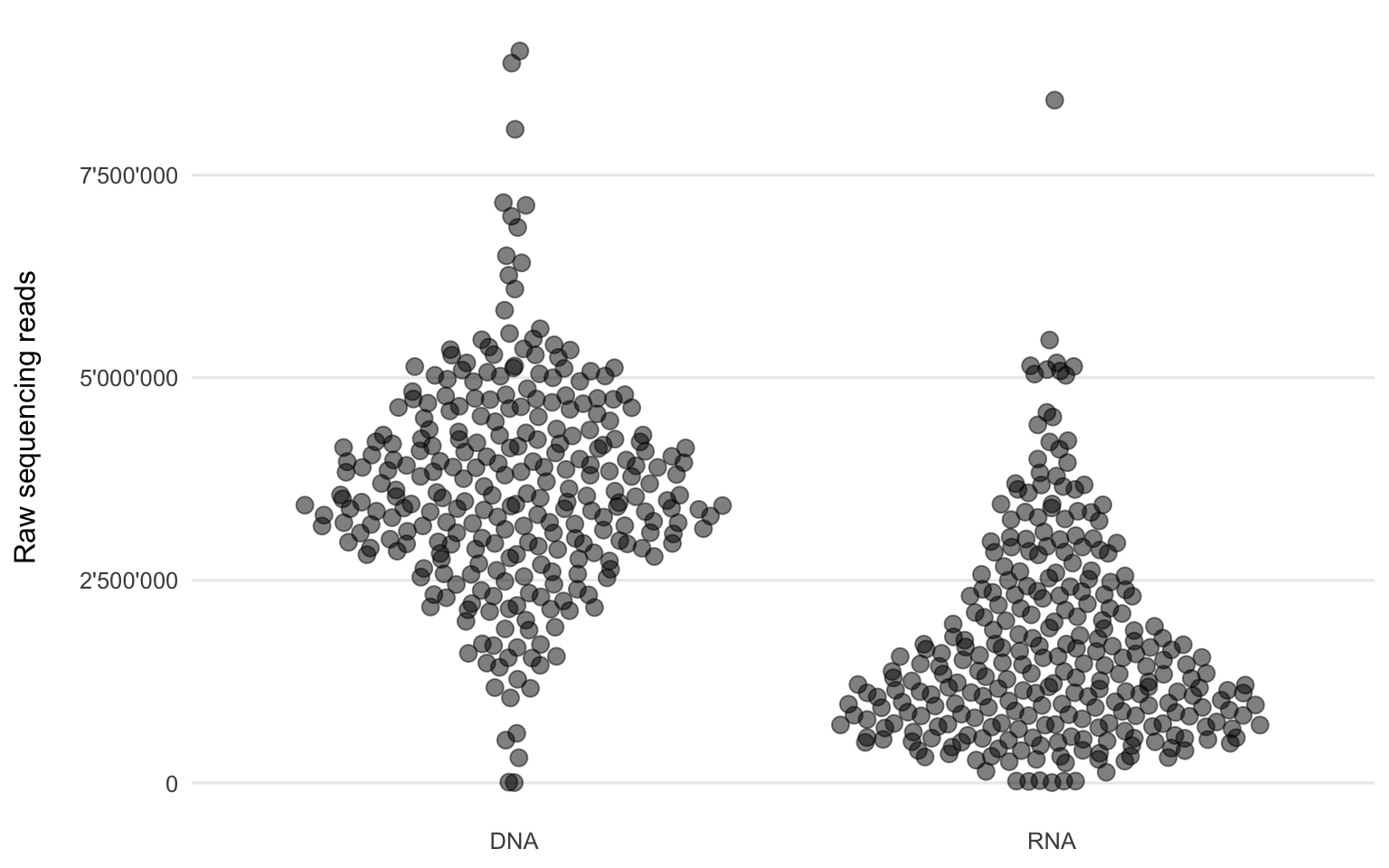
Figure 3.1: Number of raw sequencing reads of each sample from the two workflows.

Figure 3.1 shows the distribution of the short (sequenced length is 151 nt, but the sequencing reads themselves can be shorter due to adapter and quality trimming) Illumina sequencing reads per sample and workflow. The DNA workflow generally yielded more sequencing reads (mean = 3’653’241) compared to the RNA workflow (mean = 1’697’050).
Using the bioinformatic pipeline VirMet (github.com/medvir/VirMet), these sequencing reads were processed and classified. The proportions of the classes (human, bacterial, fungal, viral and unclassified) for each sample are shown in Figures 3.2 and 3.3.

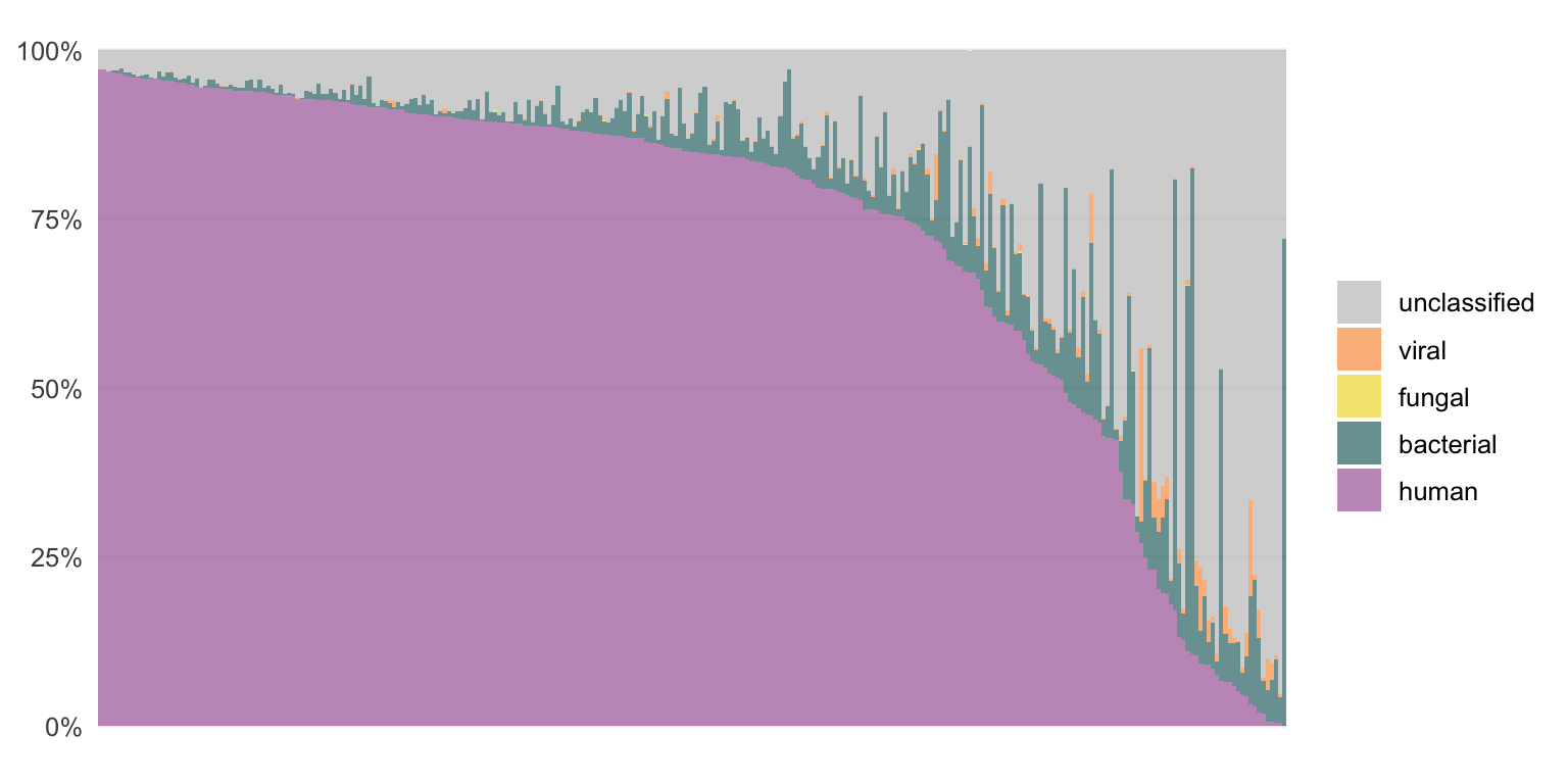
Figure 3.2: The composition of DNA samples when the sequencing reads are classified by VirMet.

Each bar represents one sample. They are ordered by the proportion of human reads to simplify the figures. Most of the DNA samples contain mainly human or unclassified reads while for the RNA samples there are mostly human or bacterial reads.
There are samples with a high fraction of viral or fungal reads which indicates an infection.

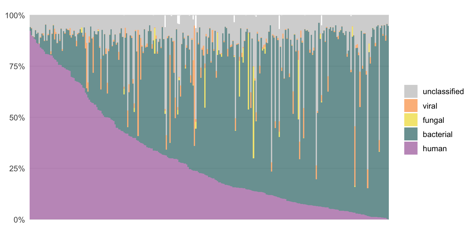
Figure 3.3: The composition of RNA samples when the sequencing reads are classified by VirMet.

3.2 Semi-supervised approach - concept

In order to classify more of the unclassified (using VirMet) reads, we proposed and tested a different, semi-supervised approach.
The schema in Figure 3.4 visualizes the idea behind this approach.

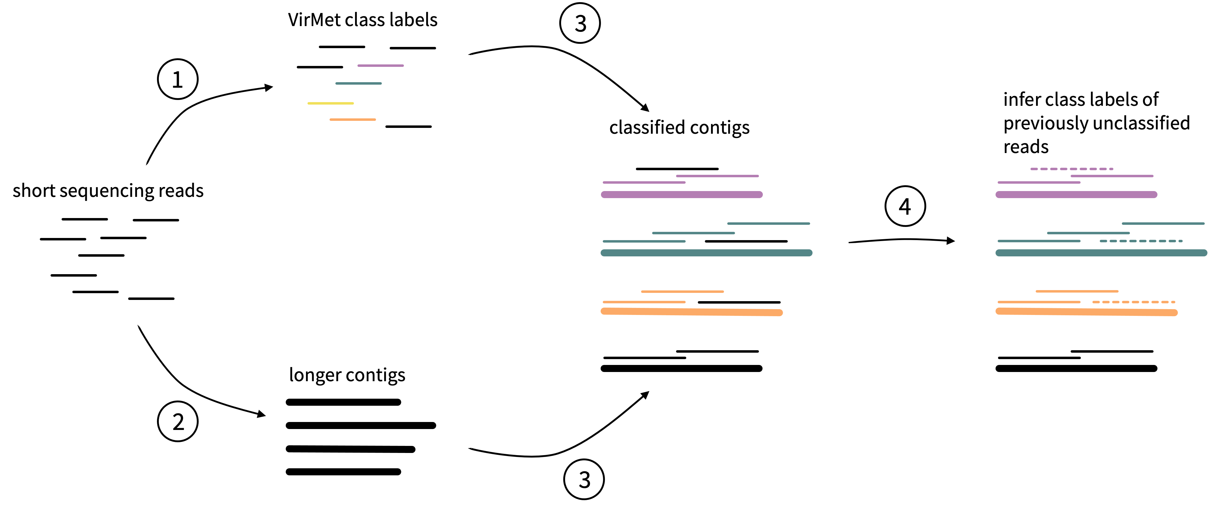
Figure 3.4: Schematic visualisation of the idea behind the semi-supervised approach to label previously unclassifed sequencing reads. Thinner lines represent the original short sequencing reads and the thicker lines longer contigs from assembly.

It can be divided into four main steps:

1. Short sequencing reads are processed and assigned class labels by VirMet. The determined class labels of the reads are represented by the colored lines in Figure 3.4. Black lines represent reads that could not be classified.
   
2. Using the metagenome assembler Megahit²⁴, longer so-called contigs are created de novo (without using reference sequences).
   
3. By mapping the short reads back to the longer contigs, the class label of the contigs can be derived by adopting the label of the by VirMet labeled reads.
   
4. The class label of the mapped but previously unclassified reads can be inferred by the contig label.

These steps, excluding running VirMet, are part of the bioinformatic Snakemake workflow which is described in Section 3.3.

3.3 Snakemake workflow

In order to make this work replicable, the code used to get the information out of the sequencing read files and the VirMet output is published on GitHub (sschmutz/thesis-workflow) in form of a Snakemake workflow.²⁵
In addition to be able to replicate the results shown here, another advantage of having a Snakemake workflow is the possibility of reusing parts (Snakemake rules) for other projects.
The code is listed in Appendix A.

3.3.1 Setup

This Section describes the steps which are required to set up this Snakemake workflow.

Get the contents of the Git repository by cloning it from GitHub:
git clone https://github.com/sschmutz/thesis-workflow.git

Edit the Snakefile by adding all names of the samples which should be processed (or import them from a file) and determine a threshold (in percent) which is applied to label the contigs in rule “infer_class_labels”.

Prepare a folder within the cloned Git repository named data/sequencing_files/ containing the compressed raw and unclassified sequencing files ({sample}.fastq.gz and {sample}_unclassified-reads.fastq.gz) for each sample that should be analysed. Creating a symbolic link instead of copying the files is also possible. Maintaining the same folder and file name structure suggested here allows that the Snakefile does not need to be adapted beyond specifying the sample names and the threshold value.
In another folder named data/virmet_dbs the fasta files of all database sequences which were used for VirMet need to be present.
The VirMet output itself has also to be prepared in a separate folder data/virmet_output where the results of each sample need to be present in a sub-folder named after the sample. Required are all cram files created during the decontamination steps of VirMet and viral_reads.fastq.gz which contains all sequencing reads which were assigned to a virus.

3.3.2 Rules

The workflow is divided into six different steps, also called rules in Snakemake and a pseudo-rule (all) which combines all rules.
Figure 3.5 shows a directed acyclic graph (DAG) which helps to visualize the rules and how they are connected by their input and output.

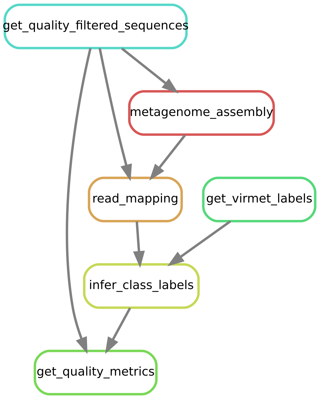
Figure 3.5: Directed acyclic graph (DAG) of the Snakemake workflow.

3.3.2.1 All

This pseudo-rule lists all files that should be created and combines all rules explained below.
Running this rule executes all processes at once for the samples and threshold value specified at the top of the Snakefile. It is the simplest way to execute the whole workflow and can be run using the following command:

snakemake --cores 4

The following output files are required to replicate the findings presented in the Results section of the thesis and are thus listed and produced by this final summarizing rule:

• Quality profiling for all samples and types (classified-reads, unclassified-reads, unclassified-in-contig-reads and unclassified-not-in-contig-reads) written to
  data/quality_metrics/{sample}_{type}.json.

• Assembly statistics (contig name, flag, multi and length) for the contigs of each sample is written to data/metagenome_assembly/{sample}_final.contigs.lst.

• The outcome of the semi-supervised approach to classify previously unclassified reads is written for each sample and specified threshold to
  data/undetermined_class_label/{sample}_{threshold}.csv.

3.3.2.2 Get quality-filtered sequences

Since there is no file containing all classified sequences among the VirMet output, it needs to be created first.
There are however files containing all raw sequences and all unclassified sequences respectively (prepared in Section 3.3.1). It is therefore possible to get the classified sequences as follows:

\[\text{raw sequences} - \text{sequences removed by QC} - \text{unclassified sequences} = \text{classified sequences}\]

Since there is also no information about the reads which failed the QC implemented in VirMet, the quality filtering steps need to be repeated.
In addition to some intermediate temporary files (which are automatically deleted after finishing this rule), the only output is a compressed fastq file named
data/sequencing_files/{sample}_classified-reads.fastq.gz which contains all classified sequencing reads for each sample.

To run this rule for a sample, the following command can be used (replace {sample} with an actual sample name):

snakemake --cores 4 data/sequencing_files/{sample}_classified-reads.fastq.gz

3.3.2.3 Metagenome assembly

All reads per sample which passed the VirMet quality filtering steps
(data/sequencing_files/{sample}_classified-reads.fastq.gz and
data/sequencing_files/{sample}_unclassified-reads.fastq.gz) are used for a metagenome assembly using Megahit²⁴ with the default parameter. Only the memory (-m) and thread (-t) usage are specified.
From the metagenome assembly, the minimum files which are needed to proceed are kept and compressed to optimize the storage space required. These are the final contigs (data/metagenome_assembly/{sample}_final.contigs.fasta.gz) and the assembly statistics (data/metagenome_assembly/{sample}_final.contigs.lst) which are the sequencing headers.
If the intermediate contigs should be kept, the temp() tag of the metagenome assembly output has to be removed.

To run this rule for a sample, the following command can be used (replace {sample} with an actual sample name):

snakemake --cores 4 data/metagenome_assembly/{sample}

3.3.2.4 Read mapping

Since during the metagenome assembly the information of which read is part of which contig is lost, all sequencing reads used for the assembly have to be mapped back to these contigs.
The read mapping is done using minimap2 with the settings for short accurate genomic reads (-ax sr). Again, to save storage space, only the minimum information required (query sequence name, target sequence name) is stored in a table (data/metagenome_assembly_read_mapping/{sample}_aln.tsv.gz). For the mapped reads, the target sequence name is the contig name to which a read mapped to, while for the unmapped reads it is an asterisk.

To run this rule for a sample, the following command can be used (replace {sample} with an actual sample name):

snakemake --cores 4 data/metagenome_assembly_read_mapping/{sample}_aln.tsv.gz

3.3.2.5 Get VirMet labels

Using VirMet, the sequencing reads are classified into different classes. The main ones considered here are: human, bacterial, fungal and viral.
For the semi-supervised approach, the labels of all classified reads are required. With the exception of the viral results, VirMet stores the alignment information in CRAM²⁶ (compressed SAM) files.
To access the information about which read mapped against which reference database by VirMet, one needs to uncompress the CRAM files. This can be done using samtools²⁷. It requires the CRAM files and the reference database (fasta file) which was used for the alignment. All mapped reads can then be written to a fastq file and by extracting just the sequence ids, a list of all reads which were aligned to a sequence of each of the classes is created.
It is a bit more straightforward for the viral reads because they are stored in fastq format (viral_reads.fastq.gz) for each sample. Only the second part of what is described in the previous paragraph, extracting the sequence ids, needs to be done to obtain the viral ids.

The output are compressed lists containing all sequence ids assigned by VirMet to the different classes.

To run this rule for a sample, the following command can be used (replace {sample} with an actual sample name):

snakemake --cores 4 data/classification/{sample}_viral.lst.gz

3.3.2.6 Infer class labels

Given a threshold value as percent, as described in Section 3.3.1, the contigs are first labeled before the class labels of previously unclassified reads are inferred.

This happens within the R script infer_class_labels.R which uses the VirMet class labels and the contig information of each sequencing read (created by the previous two rules) to infer class labels of previously unclassified reads.
The summary statistics are written to the undetermined_class_label folder and two lists of sequencing reads for the two classes “unclassified_in_contig” and “unclassified_not_in_contig” are written to the classification folder.

To run this rule for a sample, the following command can be used (replace {sample} with an actual sample name and define a {threshold} value):

snakemake --cores 4 data/undetermined_class_label/{sample}_{threshold}.csv

3.3.2.7 Get quality metrics

The bioinformatic tool fastp¹⁵ is used to get multiple quality metrics of the “classified” and “unclassified” reads separately for each sample. The “unclassified” fraction is also further subdivided into “unclassified-in-contig” and “unclassified-not-in-contig” depending on if they could be mapped to a longer contig or not. The output containing multiple quality metrics and filtering statistics is written to json files in the quality_measures folder.

To run this rule for a sample, the following command can be used (replace {sample} with an actual sample name):

snakemake --cores 4 data/quality_metrics/{sample}_classified-reads.json

3.4 Software

The following main tools were used to perform the computational analysis and for writing this thesis.

Software	Version	Reference
fastp	0.20.1	Chen et al., (2018)15
megahit	1.2.9	Li et al., (2015)24
minimap2	2.17	Li et al., (2018)28
prinseq	0.20.4	Schmieder and Edwards, (2011)29
Python	3.9.5	van Rossum, (1995)30
R	4.0.3	R Core Team, (2020)31
R - broom	0.7.5	Robinson et al., (2021)32
R - car	3.0.10	Fox and Weisberg, (2019)33
R - corrr	0.4.3	Kuhn et al., (2020)34
R - GGally	2.1.1	Schloerke et al., (2021)35
R - ggbeeswarm	0.6.0	Clarke and Sherrill-Mix, (2017)36
R - ggrepel	0.9.1	Slowikowski, (2021)37
R - ggtext	0.1.1	Wilke, (2020)38
R - glue	1.4.2	Hester, (2020)39
R - here	1.0.1	Müller, (2020)40
R - kableExtra	1.3.4	Zhu, (2021)41
R - knitr	1.31	Xie, (2021)42
R - lemon	0.4.5	Edwards, (2020)43
R - lubridate	1.7.10	Grolemund and Wickham, (2011)44
R - patchwork	1.1.1	Pedersen, (2020)45
R - scales	1.1.1	Wickham and Seidel, (2020)46
R - see	0.6.2	Lüdecke et al., (2020)47
R - tidyjson	0.3.1	Stanley and Arendt, (2020)48
R - tidymodels	0.1.2	Kuhn and Wickham, (2020)49
R - tidyverse	1.3.1	Wickham et al., (2019)50
R - xkcd	0.0.6	Torres-Manzanera, (2018)51
samtools	1.12	Danecek et al., (2021)27
seqkit	0.16.1	Wei et al., (2016)52
seqtk	1.3	Li, (2021)53
Snakemake	6.4.1	Mölder et al., (2021)25

References

15. Chen, S., Zhou, Y., Chen, Y. & Gu, J. Fastp: An ultra-fast all-in-one FASTQ preprocessor. Bioinformatics 34, i884–i890 (2018).

24. Li, D., Liu, C.-M., Luo, R., Sadakane, K. & Lam, T.-W. MEGAHIT: An ultra-fast single-node solution for large and complex metagenomics assembly via succinct de Bruijn graph. Bioinformatics (Oxford, England) 31, 1674–1676 (2015).

25. Mölder, F. et al. Sustainable data analysis with Snakemake. F1000Research 10, 33 (2021).

26. Hsi-Yang Fritz, M., Leinonen, R., Cochrane, G. & Birney, E. Efficient storage of high throughput DNA sequencing data using reference-based compression. Genome Research 21, 734–740 (2011).

27. Danecek, P. et al. Twelve years of SAMtools and BCFtools. GigaScience 10, giab008 (2021).

28. Li, H. Minimap2: Pairwise alignment for nucleotide sequences. Bioinformatics 34, 3094–3100 (2018).

29. Schmieder, R. & Edwards, R. Quality control and preprocessing of metagenomic datasets. Bioinformatics 27, 863–864 (2011).

30. Rossum, G. van. Python tutorial. (1995).

31. R Core Team. R: A language and environment for statistical computing. (R Foundation for Statistical Computing, 2020).

32. Robinson, D., Hayes, A. & Couch, S. Broom: Convert statistical objects into tidy tibbles. (2021).

33. Fox, J. & Weisberg, S. An R companion to applied regression. (Sage, 2019).

34. Kuhn, M., Jackson, S. & Cimentada, J. Corrr: Correlations in r. (2020).

35. Schloerke, B. et al. GGally: Extension to ’ggplot2’. (2021).

36. Clarke, E. & Sherrill-Mix, S. Ggbeeswarm: Categorical scatter (violin point) plots. (2017).

37. Slowikowski, K. Ggrepel: Automatically position non-overlapping text labels with ’ggplot2’. (2021).

38. Wilke, C. O. Ggtext: Improved text rendering support for ’ggplot2’. (2020).

39. Hester, J. Glue: Interpreted string literals. (2020).

40. Müller, K. Here: A simpler way to find your files. (2020).

41. Zhu, H. KableExtra: Construct complex table with ’kable’ and pipe syntax. (2021).

42. Xie, Y. Knitr: A general-purpose package for dynamic report generation in r. (2021).

43. Edwards, S. M. Lemon: Freshing up your ’ggplot2’ plots. (2020).

44. Grolemund, G. & Wickham, H. Dates and times made easy with lubridate. Journal of Statistical Software 40, 1–25 (2011).

45. Pedersen, T. L. Patchwork: The composer of plots. (2020).

46. Wickham, H. & Seidel, D. Scales: Scale functions for visualization. (2020).

47. Lüdecke, D., Ben-Shachar, M. S., Waggoner, P. & Makowski, D. See: Visualisation toolbox for ’easystats’ and extra geoms, themes and color palettes for ’ggplot2’. CRAN (2020) doi:10.5281/zenodo.3952153.

48. Stanley, J. & Arendt, C. Tidyjson: Tidy complex ’json’. (2020).

49. Kuhn, M. & Wickham, H. Tidymodels: A collection of packages for modeling and machine learning using tidyverse principles. (2020).

50. Wickham, H. et al. Welcome to the tidyverse. Journal of Open Source Software 4, 1686 (2019).

51. Torres-Manzanera, E. Xkcd: Plotting ggplot2 graphics in an xkcd style. (2018).

52. Shen, W., Le, S., Li, Y. & Hu, F. SeqKit: A Cross-Platform and Ultrafast Toolkit for FASTA/Q File Manipulation. PLOS ONE 11, e0163962 (2016).

53. Li, H. Lh3/seqtk. (2021).